February 10, 2022

Introduction to Python Data Science Tools

tutorial

coding

The goal of this introductory Python Data Science tutorial is to illustrate the most commonly used concepts and tools for beginners.

Python Collection Data Types

There are four collection data types in the Python: List/Tuple/Set/Dictionary

The difference lies in:

Ordered (indexed) vs. Unordered (un-indexed)
Mutable (the value of an item can be changed) vs. Immutable
Duplicate vs. Unique (is duplicate items allowed or not)

The definitions are as follows. You can check usage examples in Python Cheatsheet

List [...] is a collection that is ordered, mutable and allows duplicate items.
Tuple (...) is special type of list that is ordered, immutable, and allows duplicate items.
Set {...} is a collection that is unordered, immutable, with unique items.
Dictionary {key1:value1, key2:value2,...} is a collection that is unordered, mutable, with unique keys.

NOTE: Python 3.7+, dictionaries are ordered.

Numpy

Numpy is the core library for scientific computing in Python, which provides a high-performance multidimensional array objects and related tools to work with the array.

Import convention:

import numpy as np

Creating Numpy Arrays from Python Lists

Let’s try to create the following arrays from lists. Axes are the dimensions of the array. The default axis is 0, which refers to row and axis 1 refers to column, etc.

axis

# 1D array
a = np.array([2, 5, 6, 9])  

# 2D array
b = np.array([
    [3.5, 4.0, 6.5], 
    [0.4, 0.9, 4.7],
])

# 3D array
c = np.array([
    [
        [7, 1],
        [9, 4],
        [2, 3],
    ],
    [
        [4, 5],
        [0, 6],
        [8, 0],
    ],
    [
        [1, 3],
        [3, 9],
        [6, 9],
    ],
    [
        [5, 8],
        [8, 8],
        [4, 7],
    ],
])

.ndim: number of axes (dimensions) of the array
.size: total number of elements of the array
.shape: a tuple of integers that indicate the number of elements in each axis
.dtype: data type of the array

print(a.ndim, a.size, a.shape, a.dtype)
print(b.ndim, b.size, b.shape, b.dtype)
print(c.ndim, c.size, c.shape, c.dtype)

1 4 (4,) int64
2 6 (2, 3) float64
3 24 (4, 3, 2) int64

Load from Text File

Numbers can be loaded from a text file using .loadtxt().

For example, the 3d array above can be loaded from numbers.txt.zip.

By default, the delimiter is whitespace. The example below shows how to specify comma as the delimiter.

a = np.loadtxt('numbers.txt', delimiter=',')
a = a.reshape(4, 3, 2)
print(a)

[[[7. 1.]
  [9. 4.]
  [2. 3.]]

 [[4. 5.]
  [0. 6.]
  [8. 0.]]

 [[1. 3.]
  [3. 9.]
  [6. 9.]]

 [[5. 8.]
  [8. 8.]
  [4. 7.]]]

Numpy Array vs. Python List

A list can have elements of different types but Numpy array can only have elements of the same type.
Numpy array enables element-wise computing, such as adding 1 to all elements.

# element-wise computing
a = np.array([1, 2, 3, 4])
b = np.array([5, 6, 7, 8])
print(a + 2)
print(a + b)

[3 4 5 6]
[ 6  8 10 12]

Numpy array has various functions for scientific computing.

a = np.array([1, 3, 5, 9])
b = np.array([
    [3.5, 4.0, 6.5], 
    [0.4, 0.9, 4.7],
])
print(a.sum(), a.min(), a.max(), a.mean(), np.median(a), np.std(a))
print(b.sum())
 # adding rows (axis=0) and adding columns (axis=1)
print(b.sum(axis=0), b.sum(axis=1))

18 1 9 4.5 4.0 2.958039891549808
20.0
[ 3.9  4.9 11.2] [14.  6.]

A slice of a Python list is a copy while a slice of a Numpy array is a view (same way of slicing using [start:stop:step])

For list:

# slices of a Python list are copies of the list
# changing slices DOES NOT change the original list
a = [1, 2, 3, 4, 5]
b = a[2:4]
print(a, b)

b[1] = 9  # change b
print(b)
print(a)  # a does not change

[1, 2, 3, 4, 5] [3, 4]
[3, 9]
[1, 2, 3, 4, 5]

For Numpy array:

# slices of a Numpy array are views of the array
# changing the slices will change the original array!!!
c = np.array([1, 2, 3, 4, 5])
d = c[2:4]  # d is a view of c
print(d)

d[1] = 9  # change d
print(d)
print(c)  # c changed!

[3 4]
[3 9]
[1 2 3 9 5]

use np.copy() to make a copy of a numpy array:

c = np.array([1, 2, 3, 4, 5])
f = np.copy(c)  # make a copy of c
f = f[2:4]
print(f)
f[1] = 20  # change f
print(f)
print(c)  # c is not changed

[3 4]
[ 3 20]
[1 2 3 4 5]

Numpy array is way more faster than Python list for computation

Initial Placeholder Arrays

Create evenly spaced values by step value: (start, stop, step):

>>>> np.arange(1, 10, 2) 
array([1, 3, 5, 7, 9])

Create evenly spaced values by number of samples: (start, stop, num-of-samples):

>>>> np.linspace(1, 10, 5)
array([ 1.  ,  3.25,  5.5 ,  7.75, 10.  ])

Create arrays with random numbers

>>>> np.random.random((2, 3))
array([[0.65107703, 0.91495968, 0.85003858],
       [0.44945067, 0.09541012, 0.37081825]])

Create arrays with zeros and ones:

np.zeros ((2, 3))  # 2 rows 3 columns
np.ones ((2, 3, 4))  # 3D array with all ones

See more: DataCamp Numpy Cheatsheet

Pandas

Pandas is a fast, powerful, and flexible data analysis and manipulation tool.

Use the following import convention:

import pandas as pd

Pandas Series

A pandas series is a one dimensional labeled array (a Python array is only indexed but not labeled):

# a series is an array with labeled index, default to 0, 1, 2...
s = pd.Series([7, 9, 8])

0    7
1    9
2    8
dtype: int64

You can specify index labels:

# series is array with labeled index
s = pd.Series([7, 9, 8], index=['a', 'b', 'c'])

a    7
b    9
c    8
dtype: int64

You can use the label to access the element, e.g. s['c']

Pandas DataFrame

A pandas DataFrame is a two dimensional labeled data structure with columns of potentially different types:

Create a pandas dataframe from a Python dictionary:

# column names by default are keys in the dict
countries = {
    'country': ['USA', 'China', 'Japan'],
    'gdp': [20.49, 13.40, 4.97],
    'population':[331, 1439, 126],
}
df = pd.DataFrame(countries)

  country    gdp  population
0     USA  20.49         331
1   China  13.40        1439
2   Japan   4.97         126

Choose certain columns from keys:

df = pd.DataFrame(countries, columns=['country', 'gdp'])

  country    gdp
0     USA  20.49
1   China  13.40
2   Japan   4.97

Read data from CSV (Comma-separated values) files: (countries-2021.csv.zip ):

The data file is top 10 countries by GDP (in trillions) in 2021 with information on population (in millions), area (in millions square kilometer $km^2$), capital, continent.

df = pd.read_csv('countries-2021.csv')
df

          country    gdp  population  area          capital      continent
 United States  20.49      331.00  9.53  WASHINGTON D.C.  North America
         China  13.40     1439.32  9.60          Beijing           Asia
         Japan   4.97      126.48  0.38            Tokyo           Asia
       Germany   4.00       83.78  0.36           Berlin         Europe
United Kingdom   2.83       67.89  0.24           London         Europe
        France   2.78       65.27  0.64            Paris         Europe
         India   2.72     1380.00  3.29        New Delhi           Asia
         Italy   2.07       60.46  0.30             Rome         Europe
        Brazil   1.87      212.56  8.52         Brasilia  South America
        Canada   1.71       37.74  9.98           Ottawa  North America

.index: returns the index labels
.columns: returns the column names
.info(): prints information about a DataFrame including the index dtype and columns, non-null values and memory usage.

df.info()

<class 'pandas.core.frame.DataFrame'>
RangeIndex: 10 entries, 0 to 9
Data columns (total 6 columns):
 #   Column      Non-Null Count  Dtype  
---  ------      --------------  -----  
 0   country     10 non-null     object 
 1   gdp         10 non-null     float64
 2   population  10 non-null     float64
 3   area        10 non-null     float64
 4   capital     10 non-null     object 
 5   continent   10 non-null     object 
dtypes: float64(3), object(3)
memory usage: 608.0+ bytes

.describe(): prints descriptive statistics for numerical columns excluding NaN values

df.describe()

             gdp   population      area
count  10.000000    10.000000  10.00000
mean    5.684000   380.450000   4.28400
std     6.243788   549.780564   4.51295
min     1.710000    37.740000   0.24000
25%     2.232500    65.925000   0.36500
50%     2.805000   105.130000   1.96500
75%     4.727500   301.390000   9.27750
max    20.490000  1439.320000   9.98000

.head(n)/.tail(n): returns the first/last n rows (default n=5)

df.head()

           country    gdp  population  area          capital      continent
 United States  20.49      331.00  9.53  WASHINGTON D.C.  North America
         China  13.40     1439.32  9.60          Beijing           Asia
         Japan   4.97      126.48  0.38            Tokyo           Asia
       Germany   4.00       83.78  0.36           Berlin         Europe
United Kingdom   2.83       67.89  0.24           London         Europe

Selecting data in DataFrames using `[]`

Slicing a DataFrame by rows (you have to specify a range): df[start:stop]
Slicing a DataFrame by columns:
- one column: df['column name'] or if df.column_name if there are no space in the column name
- multiple columns: df[['column name1', 'column name2',...]]

# slice by rows
df[1:3]

  country    gdp  population  area  capital continent
1   China  13.40     1439.32  9.60  Beijing      Asia
2   Japan   4.97      126.48  0.38    Tokyo      Asia

# select one column
df['country']  # same as df.country

   United States
           China
           Japan
         Germany
  United Kingdom
          France
           India
           Italy
          Brazil
          Canada
Name: country, dtype: object

# select multiple columns
df[['country','gdp']]

          country    gdp
 United States  20.49
         China  13.40
         Japan   4.97
       Germany   4.00
United Kingdom   2.83
        France   2.78
         India   2.72
         Italy   2.07
        Brazil   1.87
        Canada   1.71

Selecting data in DataFrames using `.loc[]` and `.iloc[]`

[] can only do simple data selections by rows and columns. More complicated data selection can be done by using the following methods:

.iloc[] is primarily integer position based (from 0 to length-1 of the axis)

# select rows with index 1, 4, and 6
df.iloc[[1, 4, 6]]

# here 1 and 4 are treated as indexes
# row 4 is NOT included, i.e. UK
df.iloc[1:4, :2]

   country    gdp
1    China  13.40
2    Japan   4.97
3  Germany   4.00

.loc[] is primarily label based - NOTE: even numbers are treated as labels!

# here 1 adn 4 are treated as labels
# row 4 is included, i.e. UK
df.loc[1:4, ['country', 'gdp']]  

          country    gdp
1           China  13.40
2           Japan   4.97
3         Germany   4.00
4  United Kingdom   2.83

Filtering Rows using Masking Expressions

Filtering using one expression: df[expression 1]: one expression

# returns countries with GDP greater than 3 trillions
df[df['gdp'] > 3]

         country    gdp  population  area          capital      continent
0  United States  20.49      331.00  9.53  WASHINGTON D.C.  North America
1          China  13.40     1439.32  9.60          Beijing           Asia
2          Japan   4.97      126.48  0.38            Tokyo           Asia
3        Germany   4.00       83.78  0.36           Berlin         Europe

Filtering using multiple expressions:
- df[(expression 1) & (expression 2) & ...]: multiple masking conditions with AND relationship
- df[(expression 1) | (expression 2) |...]: multiple masking conditions with OR relationship

# returns countries with GDP greater than 2 trillions and population less than 100 millions
df[(df['gdp'] > 2) & (df['population'] < 100)]

          country   gdp  population  area capital continent
3         Germany  4.00       83.78  0.36  Berlin    Europe
4  United Kingdom  2.83       67.89  0.24  London    Europe
5          France  2.78       65.27  0.64   Paris    Europe
7           Italy  2.07       60.46  0.30    Rome    Europe

Derived Columns

You can derive new columns from existing ones:

# calculate GDP per capita (GDP divided by population)
# a trillion has 12 zeros, a million has 6 zeros
df['gdp_per_capita'] = df.gdp * 1000000 / df.population
df

          country    gdp  population  area          capital  gdp_per_capita
0   United States  20.49      331.00  9.53  WASHINGTON D.C.    61903.323263
1           China  13.40     1439.32  9.60          Beijing     9309.951922
2           Japan   4.97      126.48  0.38            Tokyo    39294.750158
3         Germany   4.00       83.78  0.36           Berlin    47744.091669
4  United Kingdom   2.83       67.89  0.24           London    41685.078804
5          France   2.78       65.27  0.64            Paris    42592.308871
6           India   2.72     1380.00  3.29        New Delhi     1971.014493
7           Italy   2.07       60.46  0.30             Rome    34237.512405
8          Brazil   1.87      212.56  8.52         Brasilia     8797.515995
9          Canada   1.71       37.74  9.98           Ottawa    45310.015898

Pandas Functions

.min(), .max(), .mean(), .sum(), etc.

df.max()

country             United States
gdp                         20.49
population                1439.32
area                         9.98
capital           WASHINGTON D.C.
continent           South America

.value_counts(): return a Series containing counts of unique rows in the DataFrame.

df.continent.value_counts()  # this is a Series

Europe           4
Asia             3
North America    2
South America    1
Name: continent, dtype: int64

df.continent.value_counts()['Asia']

3

df.continent.value_counts(normalize=True)

Europe           0.4
Asia             0.3
North America    0.2
South America    0.1
Name: continent, dtype: float64

.nunique(): return Series with number of distinct elements

df.nunique()

country           10
gdp               10
population        10
area              10
capital           10
continent          4
dtype: int64

Sorting

.sort_values() can be used to sort the values, which returns a sorted DataFrame with original DataFrame unchanged.

use by='column name' or by=['column 1', column 2'] to specify columns to sort
use ascending=False to change ascending vs. descending
use ignore_index=True to label the result with index: 0, 1, …, n - 1.
use inplace=True to make the change to the DataFrame in place

# after the following line the df is NOT changed
# the index is NOT reset 
df.sort_values(by='population', ascending=False)

          country    gdp  population  area          capital      continent
         China  13.40     1439.32  9.60          Beijing           Asia
         India   2.72     1380.00  3.29        New Delhi           Asia
 United States  20.49      331.00  9.53  WASHINGTON D.C.  North America
        Brazil   1.87      212.56  8.52         Brasilia  South America
         Japan   4.97      126.48  0.38            Tokyo           Asia
       Germany   4.00       83.78  0.36           Berlin         Europe
United Kingdom   2.83       67.89  0.24           London         Europe
        France   2.78       65.27  0.64            Paris         Europe
         Italy   2.07       60.46  0.30             Rome         Europe
        Canada   1.71       37.74  9.98           Ottawa  North America

df1 = df.sort_values(by='population', ascending=False, ignore_index=True)
df1  # the index is reset 

          country    gdp  population  area          capital      continent
         China  13.40     1439.32  9.60          Beijing           Asia
         India   2.72     1380.00  3.29        New Delhi           Asia
 United States  20.49      331.00  9.53  WASHINGTON D.C.  North America
        Brazil   1.87      212.56  8.52         Brasilia  South America
         Japan   4.97      126.48  0.38            Tokyo           Asia
       Germany   4.00       83.78  0.36           Berlin         Europe
United Kingdom   2.83       67.89  0.24           London         Europe
        France   2.78       65.27  0.64            Paris         Europe
         Italy   2.07       60.46  0.30             Rome         Europe
        Canada   1.71       37.74  9.98           Ottawa  North America

GroupBy

.groupby() can be used to group the data by different values of one or more categorical columns, then various aggregation functions can be applied to each group.

df.groupby('continent')  # this returns a DataFrameGroupBy object

<pandas.core.groupby.generic.DataFrameGroupBy object at 0x11bff9310>

Sum of GDP, Population, and Area for countries in each continent:

df.groupby('continent').sum()

                 gdp  population   area
continent                                              
Asia           21.09     2945.80  13.27
Europe         11.68      277.40   1.54
North America  22.20      368.74  19.51
South America   1.87      212.56   8.52

# this returns the max in each group for each column
# for Strings max() returns highest alphabetical character
# for example: Japan's GDP is NOT 13.40
df.groupby('continent').max()

                     country    gdp  population  area          capital 
continent                                                                 
Asia                    Japan  13.40     1439.32  9.60            Tokyo   
Europe         United Kingdom   4.00       83.78  0.64             Rome   
North America   United States  20.49      331.00  9.98  WASHINGTON D.C.   
South America          Brazil   1.87      212.56  8.52         Brasilia

df.groupby('continent') returns a tuple with two elements:

the first one is the group label, such as ‘Asia’, ‘Europe’, etc.
the second one is the DataFrame for the group

The following example shows how to loop over the groups:

for group, group_df in df.groupby('continent'):
    print(group)
    print('#' * 15)
    print(group_df)
    print('-' * 60)

Asia
###############
  country    gdp  population  area    capital continent
1   China  13.40     1439.32  9.60    Beijing      Asia
2   Japan   4.97      126.48  0.38      Tokyo      Asia
6   India   2.72     1380.00  3.29  New Delhi      Asia
------------------------------------------------------------
Europe
###############
          country   gdp  population  area capital continent
3         Germany  4.00       83.78  0.36  Berlin    Europe
4  United Kingdom  2.83       67.89  0.24  London    Europe
5          France  2.78       65.27  0.64   Paris    Europe
7           Italy  2.07       60.46  0.30    Rome    Europe
------------------------------------------------------------
North America
###############
         country    gdp  population  area          capital      continent
0  United States  20.49      331.00  9.53  WASHINGTON D.C.  North America
9         Canada   1.71       37.74  9.98           Ottawa  North America
------------------------------------------------------------
South America
###############
  country   gdp  population  area   capital      continent
8  Brazil  1.87      212.56  8.52  Brasilia  South America
------------------------------------------------------------

Deletion

.drop() can be used to delete rows or columns (use inplace=True if you want the df to be altered):

df.drop([1, 3, 4])  # delete discrete rows with index 1, 3, 4, default axis=0
df.drop(df.index[3:5])  # delete middle rows
df.drop(['gdp', 'area'], axis=1)  # delete 'gdp' and 'area' columns
df.drop(['population'], axis=1, inplace=True)  # delete 'population' column in place

.reset_index(drop=True) can be used to reset the index from 0 after deletion if needed. drop=True will delete the old index.

Matplotlib

Matplotlib is a comprehensive library for creating visualizations in Python. Version 3.5.1 is used for this tutorial.

Check the version:

import matplotlib
matplotlib.__version__

Basic Matplotlib Concepts

The following picture shows the basic Matplotlib concepts:

Figure: the top level container for all the plot elements, which may contain 1 or more Axes.
Axes: an area where points can be specified in terms of x-y coordinates
Axis, Title, Label, Tick, Marker, Legend are self-explanatory

matplotlib.pyplot is a collection of functions that make matplotlib work like MATLAB.

import matplotlib.pyplot as plt

Create a figure with one axes:

fig, ax = plt.subplots()  # Create a figure containing a single axes.
x = [1, 2, 3, 4]
y = [1, 4, 2, 3]
ax.plot(x, y);  # Plot some data on the axes.

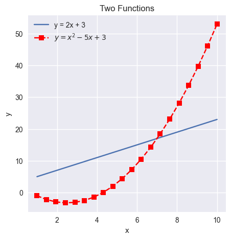
In the next example, I illustrate the followings:

create data using Numpy for plotting
set different style sheets
use figsize=(5, 5) to change the size of the plot - default is (6.4, 4.8)
specify legend labels (in plain text and LaTex)
use different line styles
use different marker styles
specify colors
set ticks and tick lables: by default the tick and tick labels are automatically generated. ax.set_xticks() and ax.set_yticks() can be used to customize the ticks and tick labels. For example, ax.set_xticks([1, 3, 7, 8], ['a', 'b', 'c', 'd']) set 4 ticks with corresponding labels for the x-axis.
set plot title
set axis labels

import numpy as np
plt.style.use('seaborn')  # seaborn style, which looks better than the default one
# plt.style.use('default')  # reset to default style

x = np.linspace(1, 10, 20)  # return 20 evenly spaced numbers between 0 and 10
y1 = 2 * x + 3  # a linear function
y2 = x**2 - 5 * x + 3  # a quadratic function

fig, ax = plt.subplots(figsize=(5, 5))  # one axes of size (5, 5)
ax.plot(x, y1, label='y = 2x + 3')
ax.plot(x, 
        y2, 
        label='$y = x^2 - 5x + 3$',  # legend label using Latex
        linestyle='dashed',  # line style
        marker='s',  # marker style
        color='red', # line color
        )

ax.set_title('Two Functions')  # plot title
ax.set_xlabel('x')  # x label
ax.set_ylabel('y')  # y label
# ax.set_xticks([1, 3, 7, 8], ['a', 'b', 'c', 'd'])  # change the x ticks and labels
ax.legend()  # show legend

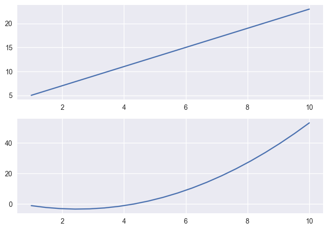
Multiple Axes

A figure can have multiple axes:

one column/one row of axes: use ax[0], ax[1], … to refer to the axes.

fig, ax = plt.subplots(2)  # two rows
ax[0].plot(x, y1)
ax[1].plot(x, y2)

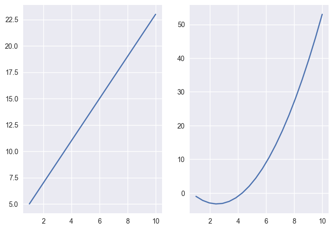
fig, ax = plt.subplots(1, 2)  # one row, two columns
ax[0].plot(x, y1)
ax[1].plot(x, y2)

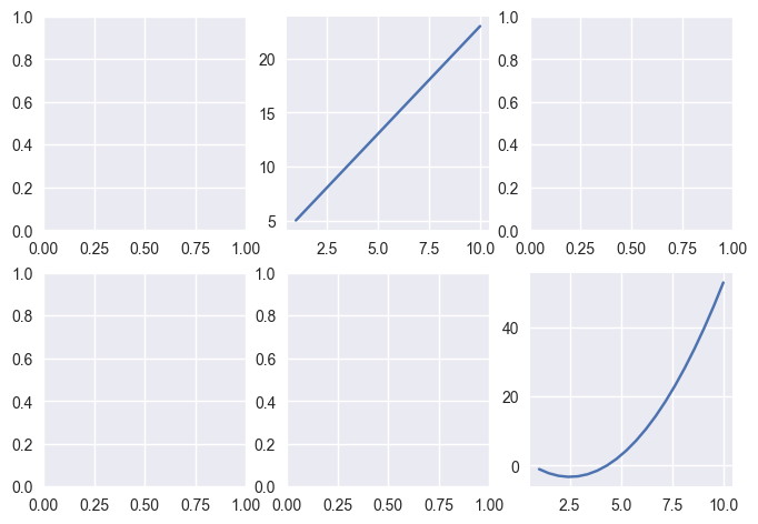
multiple rows and columns: must use ax[row, column], such as ax[0, 0], ax[0, 1], ax[1, 0], … to refer to the axes.

fig, ax = plt.subplots(2, 3)  # 2 rows and 3 columns
ax[0, 1].plot(x, y1)
ax[1, 2].plot(x, y2)

Pandas Charting

Pandas charting is built on top of Matplotlib.

I will use Country GDP dataset (countries-2021.csv.zip) and California housing dataset (housing.csv.zip) to illustrate the charts. You can learn more about the dataset from my Kaggle dataset page.

We introduce the following plots:

Line Plot
Bar Plot
Histogram
Box Plot
Scatter Plot
Scatter Matrix

Line Plot

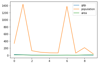
.plot() (same as .plot.line()) is used to create line plots for all numerical columns with x-axis being the number of rows

import pandas as pd
df_country = pd.read_csv('countries-2021.csv')
df_country.plot()

df_country.plot() is same as the following (figure and axis are implicitly created and used):

fig, ax = plt.subplots()
df_country.plot(ax=ax)

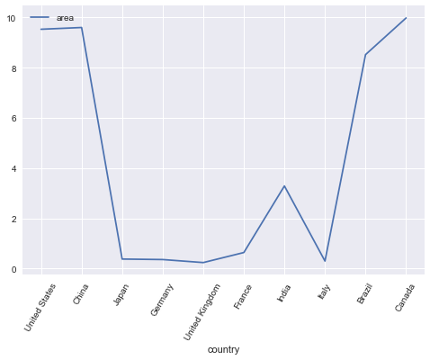
Change the style sheet and only plot one column (country area) with custom ticks:

import matplotlib.pyplot as plt
plt.style.use('seaborn')

df_country.area.plot().set_xticks(df_country.index, df_country.country, rotation=60)

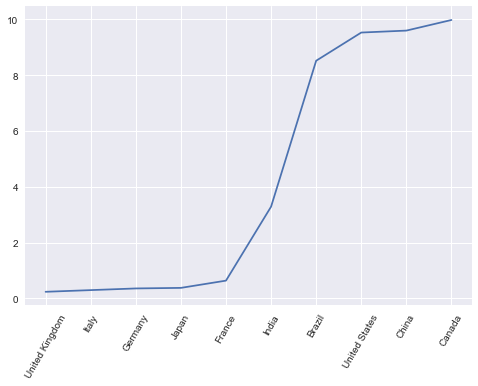
Create a new sorted DataFrame and plot the area with tick labels (ignore_index=True reset the index from 0):

df_sorted_area = df_country.sort_values(by='area', ignore_index=True)
df_sorted_area.area.plot().set_xticks(df_sorted_area.index, df_sorted_area.country, rotation=60)

Read the California housing dataset:

import pandas as pd
df_housing = pd.read_csv('housing.csv')
df_housing.info()

RangeIndex: 20640 entries, 0 to 20639
Data columns (total 10 columns):
 #   Column              Non-Null Count  Dtype  
---  ------              --------------  -----  
 0   longitude           20640 non-null  float64
 1   latitude            20640 non-null  float64
 2   housing_median_age  20640 non-null  float64
 3   total_rooms         20640 non-null  float64
 4   total_bedrooms      20433 non-null  float64
 5   population          20640 non-null  float64
 6   households          20640 non-null  float64
 7   median_income       20640 non-null  float64
 8   median_house_value  20640 non-null  float64
 9   ocean_proximity     20640 non-null  object 
dtypes: float64(9), object(1)

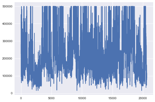
Create a line plot for the median house price - think about what patterns you can see from this line chart?

df_housing.median_house_value.plot()

Bar Plot

Bar plot shows a bar for each data point (whereas a line plot uses lines to connect the data points).

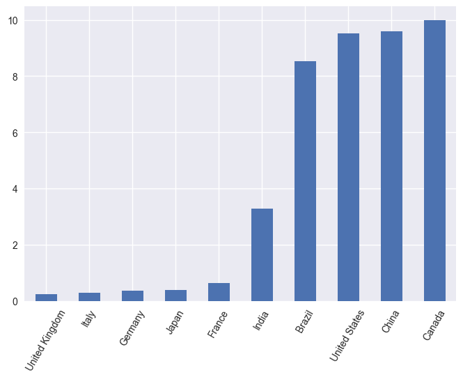
We can show the DataFrame on countries sorted by area as a bar plot:

df_sorted_area.area.plot.bar().set_xticks(df_sorted_area.index, df_sorted_area.country, rotation=60)

Histogram

.hist() (same as .plot.hist()) is often used to create histograms to check the followings:

The distributions of the data
center and spread of the data
skewness of the data
presence of outliers

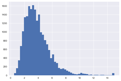
bins=50 can be used to change the number of bins, default is 10

# numerical data
df_housing.median_income.hist(bins=50)

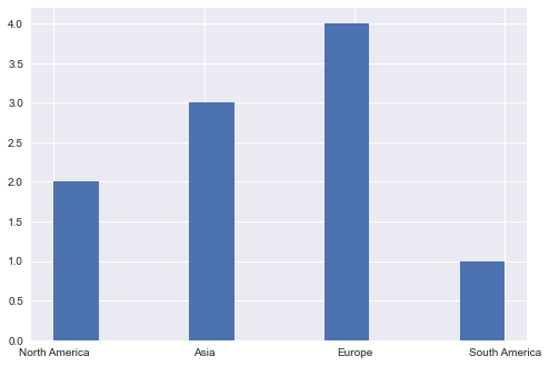
# categorical data
df_country.continent.hist()

Boxplot

A box plot .plot.box() shows:

the median (the line in the box)
the middle 50% of the data (the box)
the outliers (the dots)
smallest and largest data points after removing outliers

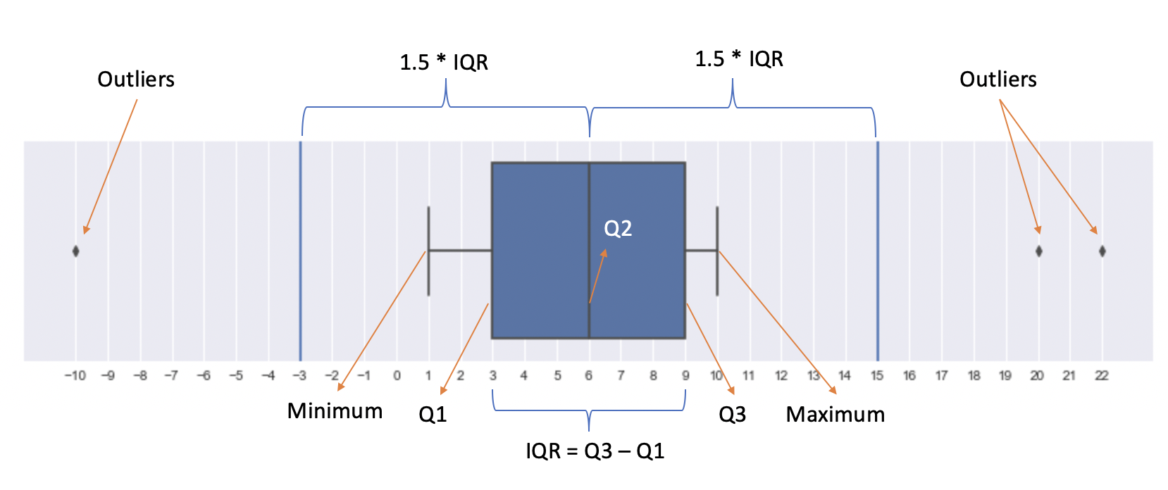
The box plot is constructed in the following steps:

find the median (the middle value of the dataset or Q2/50th Percentile) of the dataset and divide the data into lower half (smaller numbers) and upper half (larger numbers)
find the median of the lower half of the dataset, which is called Q1 (First quartile/25th Percentile)
find the median of the upper half of the dataset, which is called Q3 (Third quartile/75th Percentile)
Calculate IQR (Interquartile Range): IQR = Q3 - Q1
Identify outliers (if any): data points that are 1.5 IQR away from the median are considered outliers
remove the outliers from the dataset and minimum/maximum is the smallest/largest number in the remaining dataset

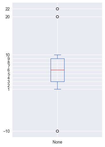
The following example shows how a boxplot is constructed step by step:

13 numbers in total, median is 6
Q1 is 3: the median of [-10, 1, 2, 3, 4, 5]
Q3 is 9: the median of [7, 8, 9, 10, 20, 22]
IQR is 9 - 3 = 6 and 1.5 IQR is 1.5 * 6 = 9
1.5 IQR from the median is -3 (6 - 9) and 15 (6 + 9), so -10, 20, 22 are outliers
minimum/maximum is then 1/10

s = pd.Series([-10, 1, 2, 3, 4, 5, 6, 7, 8, 9, 10, 20, 22])
fig, ax = plt.subplots(figsize=(4, 6))
s.plot.box()
ax.set_yticks(s)

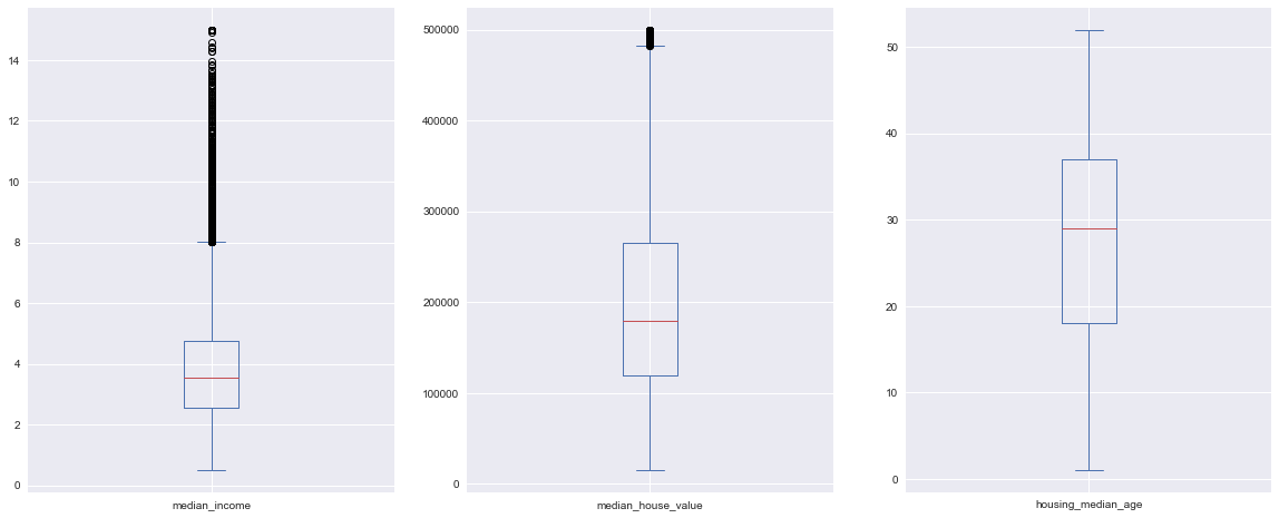
The following example also shows how to have multiple axes for different pandas charts:

fig, ax = plt.subplots(1, 3, figsize=(20,8))
df_housing.median_income.plot.box(ax=ax[0])  # income
df_housing.median_house_value.plot.box(ax=ax[1])  # house price
df_housing.housing_median_age.plot.box(ax=ax[2])  # house age

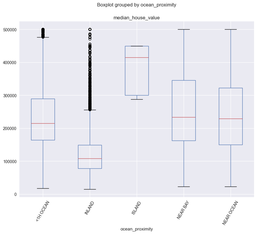
You can also show the boxplots for one feature/column for different groups (like using groupby):

df_housing.boxplot(column=['median_house_value'], by='ocean_proximity', figsize=(10, 8), rot=60)

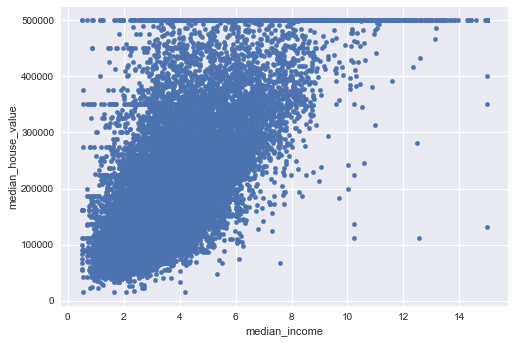
Scatter Plot

Scatter plot .plot.scatter() is often used for correlation analysis between different features. Correlation coefficient is between -1 and 1, representing negative and positive correlations. 0 means there is no liner correlation. Correlation is said to be linear if the ratio of change is constant, otherwise is non-linear.

What insights you can get from the following scatter plot?

df_housing.plot.scatter(x='median_income', y='median_house_value')

Create a scatter matrix (histogram plots in the diagonal):

pd.plotting.scatter_matrix(df_housing, figsize=(25,25))